

I was reminiscing early this week about the days that I just spent hours in Tableau with Wyscout data and making scatterplots for the life of it. I think Twitter specifically saw more scatterplots than ever before from football data enthusiasts. Then, it made me think: how did we try to find the best performing players?
Immediately, my mind turns toward outliers. It’s a way to look for the players that stand out in certain metrics. One of my favourite pieces on outliers is this one by Andrew Rowlin:
Finding Unusual Football Players – update 2024 – numberstorm blog
Outlier detection for football player recruitment an update
In this article, I will focus on a few things:
- What are outliers in data?
- Anomalies: contextual anomaly
- Data
- Methodology
- Exploratory data visualisation
- Final thoughts
Outliers
Outliers are data points that significantly deviate from most of the dataset, such that they are considerably distant from the central cluster of values. They can be caused by data variability, errors during experimentation or simply uncommon phenomena which occur naturally within a set of data. Statistical measures based on interquartile range (IQR) or deviations from the mean, i.e. standard deviation, are used to identify outliers.
In a dataset, an outlier is defined as one lying outside either 1.5 times IQR away from either the first quartile or third quartile, or three standard deviations away from the mean. These extreme figures may distort analysis and produce false statistical conclusions thereby affecting the accuracy of machine learning models.
Outliers require careful treatment since they can indicate important anomalies worth further investigation or simply result from collecting incorrect data. Depending on context, these can be eliminated, altered or algorithmically handled using certain techniques to minimize their effects. In sum, outliers form part of the crucial components used in data analysis requiring an accurate identification and proper handling to make sure results obtained are strong and dependable.
Anomalies
Anomalies in data refer to data points or patterns that deviate significantly from the expected or normal behavior, often signaling rare or exceptional occurrences. They are distinct from outliers in that anomalies often refer to unusual patterns that may not be isolated to a single data point but can represent a broader trend or event that warrants closer examination. These anomalies can arise due to various reasons, including rare events, changes in underlying systems, or flaws in data collection or processing methods.
Detecting anomalies is a critical task in many domains, as they can uncover important insights or highlight errors that could distort analysis. Statistical methods such as clustering, classification, or even machine learning techniques like anomaly detection algorithms are often employed to identify such deviations. In addition to traditional methods, time series analysis or unsupervised learning approaches can be used to detect shifts in patterns over time, further enhancing the detection of anomalies in dynamic datasets.
Anomalies are often indicators of something noteworthy, whether it’s a significant business event, a potential fraud case, a technical failure, or an unexpected change in behavior. Therefore, while they can sometimes represent data errors or noise that need to be cleaned or corrected, they can also reveal valuable insights if analysed properly. Just like outliers, anomalies require careful handling to ensure that they are properly addressed, whether that means investigating the cause, adjusting the data, or utilising algorithms designed to deal with them in the context of the larger dataset.
Contextual anomaly
There are three main types of anomalies: point anomalies, contextual anomalies, and collective anomalies. Point anomalies, also known as outliers, are individual data points that deviate significantly from the rest of the dataset, often signaling errors or rare events. Contextual anomalies are data points that are unusual in a specific context but may appear normal in another. These anomalies are context-dependent and are often seen in time-series data, where a value might be expected under certain conditions but not others. Collective anomalies, on the other hand, occur when a collection of related data points deviates collectively from the norm, even if individual points within the group do not seem anomalous on their own.
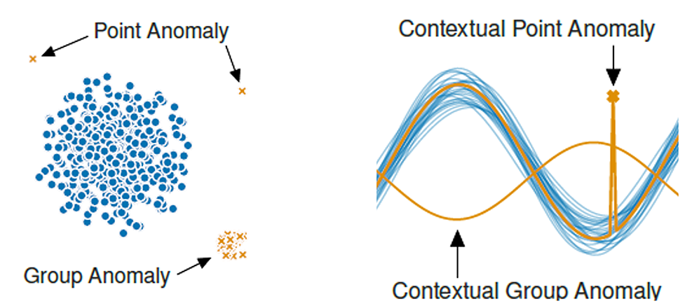
For my research, I will focus on contextual anomalies. A contextual anomaly is when a data point is unusual only in a specific context but may not be an outlier in a general sense. As we have already written and spoken about outliers, I will focus on contextual anomaly in this article.
Data
The data I’m using for this part of data scouting comes from Wyscout/Hudl. It was collected on March 23rd, 2025. It focuses on 127 leagues, of which three different seasons are featured: 2024, 2024–2025 and if there are enough minutes: 2025 season. The data is downloaded with all stats to have the most complete database.
I will filter for position as I’m only interested in strikers, so I will look at every player that has position = CF or has one of their positions as CF. Next to that, I will look at strikers who have played at least 500 minutes through the season, as that gives us a big enough sample over that particular season and a form of representative value of the data.
Methodology
Before we go into the actual calculation for what we are looking for, it’s important to get the right data from our database. First, we need to define the context and anomaly framework:
- The context variable: In this example, we use xG per 90
- The target variable: what do we want to know? Is whether a player overperforms or underperforms their xG, so we set Goals per 90 as the target variable
- Contextual anomaly: When Goals per 90 > xG per 90 + threshold, but only when xG per 90 is low
How does this look in the code for Python, R and Julia?df_analysis[‘Anomaly Score’] = df_analysis[‘Goals per 90’] – df_analysis[‘xG per 90’]
# Define contextual anomaly threshold
anomaly_threshold = 0.25
low_xg_threshold = 0.2
# Flag contextual anomalies
anomalies = df_analysis[
(df_analysis[‘Anomaly Score’] > anomaly_threshold) &
(df_analysis[‘xG per 90’] < low_xg_threshold)
]
# Calculate Anomaly Score
df_analysis <- df_analysis %>%
mutate(Anomaly_Score = `Goals per 90` – `xG per 90`)
# Define thresholds
anomaly_threshold <- 0.25
low_xg_threshold <- 0.2
# Flag contextual anomalies
anomalies <- df_analysis %>%
filter(Anomaly_Score > anomaly_threshold & `xG per 90` < low_xg_threshold)
# Calculate Anomaly Score
df_analysis.Anomaly_Score = df_analysis.”Goals per 90″ .- df_analysis.”xG per 90″
# Define thresholds
anomaly_threshold = 0.25
low_xg_threshold = 0.2
# Flag contextual anomalies
anomalies = filter(row -> row.Anomaly_Score > anomaly_threshold && row.”xG per 90″ < low_xg_threshold, df_analysis)
What I do here is set the low xG threshold for 0,2. You can alter that of course, but I find that if you put it higher it will give much more positive anomalies than perhaps might be useful for your research.\
You can also do it statistically and work with z-scores. It will then ask you to give how many standard deviations from the mean will be classified as an anomaly. This is similar to my approach with outliers:
Using a standard deviation, we look at the best-scoring classic wingers in the Championship, using the standard deviation and comparing them to the age. The outliers are calculated as being +2 from the mean and are marked in red.
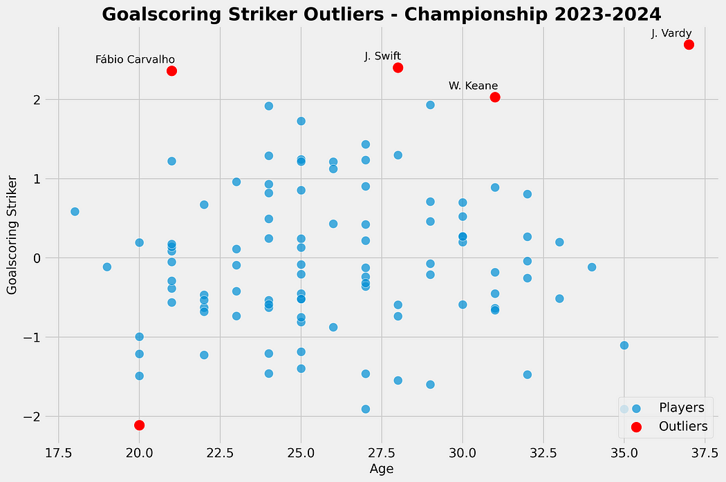
As we can see in our scatterplot, we see Carvalho, Swift, Keane and Vardy as outliers in our calculation for the goalscoring striker role score. They all score above +2 above the mean, and this is done with the calculation for Standard Deviation.
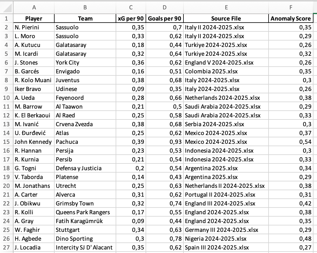
Okay, back to anomalies! Now we have our dataframe for all strikers in our database that have played at least 500 minutes with the labels: other players and anomalies. We save this to an Excel, JSON or CSV file — so it’s easier to work with.
Data visualisation
In essence an anomaly in this context is when a player has low(er) xG but has significantly higher Goals. We can show what this looks like through two visuals:
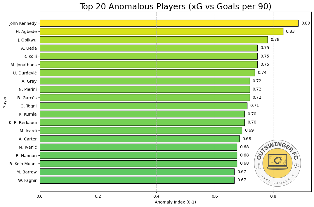
In the bar chart above, you can see the top 20 players based on anomaly index. John Kennedy for example, has the highest anomaly index, meaning that he scores highest on a high goal vs low xG ratio. This allows us to visualise what the top players are in this metric.
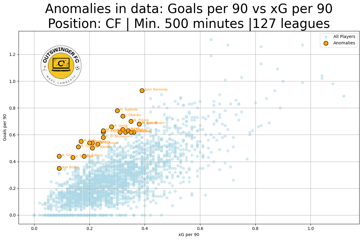
In this scatterplot you can find all players that are within our criteria. As you can see the blue dots are non-anomaly players and the orange ones are the anomaly players. What we can see here is that for a certain xG per 90 the anomalies have a higher Goal per 90.
In this way, we can have a look at how anomalies are interesting to track for scouting, but is important to ask yourself a critical question: how sustainable is their overperformance?
Final thoughts
Anomaly data scouting could be used more. It’s all about finding those players who really stand out from the crowd when it comes to their performance stats. By diving into sophisticated statistical models and getting a little help from machine learning, Scouts can spot these hidden gems — players who might be flying under the radar but are killing it.
This way of doing things gives clubs a solid foundation to make smarter decisions, helping them zero in on players who are either outperforming what folks expect or maybe just having a streak of good luck that won’t last. Anomaly detection is especially handy when it comes to scouting for new signings, figuring out who should be in the starting lineup, and even sizing up the competition. But don’t forget, context is key — stuff like the team’s playing style, strategies, and other outside factors really need to be taken into account along with the data.
At the end of the day, anomaly detection isn’t some magic wand that’ll solve everything, but it’s definitely a powerful tool.