

Data metrics and development always feel or look innovative. About 40% of the time, they are. It is very satisfying to create something that completely suits your needs, but one question always remains: how necessary is it to do so? My reason for it is that some metrics already exist, and it isn’t always necessary for your analysis to create everything yourself. It’s very time-consuming, and that’s not something we analysts often have.
To me, there is one clear exception: you don’t have the right resources. Often, we can look at event data and create our metrics, indexes and models from there. However, sometimes we want to look at off-ball data and we need tracking data to generate positional data and off-ball runs, for example. I’m quite fortunate to work with clubs that have access to that data, but what if you don’t have that? You want to use the event data to be creative and give an indication of what is close to tracking data.
This might sound familiar to you, reading this or the concept from it. We do love pressing data, but not all providers have that, so we have a metric that measures pressing intensity: Passes Per Defensive Action (PPDA). It calculates the number of passes allowed by a team’s opponent before the pressing team makes a defensive action (like a tackle, interception, or foul) in the opponent’s defensive two-thirds of the pitch. A low PPDA means aggressive pressing, and a lower PPDA means a more passive pressing approach.
In this article, I want to calculate a way to get third-man runs data with event data. After that, I want to evaluate how sound this method is and how reliable the results are.
Contents
- Why this research?
- Data collection
- Methodology
- Calculation
- Analysis
- Checks and evaluation
Why this research
This research is twofold, actually. My main aim is to see if I can find a creative way to capture third man runs with event data. I think it will give us some off-ball data via an out-of-the-box thinking pattern. Then we can use this in terms of off-ball scouting, analysis of players and teams, and of course, we can go even further and make models of that that predict a third-man run.
The second reason is that I feel that I can do better with evaluating the things I make. Check myself, check the validity of the models and the representation of the data. If I build this more into my public work, it will lead to a better understanding of the data engineering process, which is often frustrating and takes a long time to get right.
Data collection
The data collection is almost the same as in all other projects. The data I’m using is even data from Opta/Statsperform, which means it contains the XY-values of every on-ball data as collected by this specific provider.
The data has been collected on Saturday, 12th of April 2025. The data concentrates on one league specifically, and that is the Argentinian League 2025, as I’m branching out to South American football content only on this platform.
What I also will aim to do is to create a few new metrics, which will then be my own metrics. These are my designs based on Opta/Statsperform data and will be available on my GitHub page.
Methodology
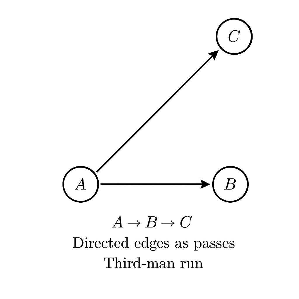
Third man runs are one of football’s most elegant attacking patterns — subtle, intelligent, and often decisive. At their core, these movements involve three players: the first (Player A) plays a pass into a teammate (Player B), who quickly connects with a third player (Player C) arriving from a different area. It’s C who truly benefits, receiving the ball in space created by the initial pass-and-move. This movement structure mirrors the concept of triadic closure from network theory, where three connected nodes form a triangle — a configuration known to create stability and flow in complex systems. In football, this triangle is a strategic weapon: it preserves possession while simultaneously generating overloads and disorganizing defensive shapes.
To detect these patterns in event data, we treat each pass as a directed edge in a dynamic graph, with time providing the sequence. The detection algorithm follows a constrained path: A→B followed by B→C, where A, B, and C are distinct teammates. The off-ball movement from A’s pass to C’s reception is measured using Euclidean distance — a direct application of spatial geometry to quantify run intensity. But there’s more at play than just movement. From an information-theoretic perspective, third man runs are low-probability, high-reward decisions. Using Shannon entropy, we can frame each player’s passing options as a probability distribution: the higher the entropy, the more unpredictable and creative the decision. Third man runs often emerge in moments of lower entropy, where players bypass obvious choices in favor of coordinated, rehearsed sequences.
Over time, these passing sequences can be modeled as a Markov chain, where each player’s action (state) depends only on the previous action in the chain. While simple possession patterns often result in high state recurrence (e.g., passing back and forth), third man runs introduce state transitions that break the chain’s memoryless monotony. This injects volatility and forward momentum into the system — qualities typically associated with higher goal probability. By combining network topology, geometric analysis, and probabilistic modeling, we build not just a detector but a lens into one of football’s most intelligent tactical tools. And with a value-scoring mechanism grounded in normalization and vector calculus, we begin to quantify what coaches have always known: the most dangerous player is often the one who never touched the ball until the moment it mattered.
Calculations
Let’s walk through how we identify and evaluate a third-man run using real match data. Imagine Player A, a midfielder, passes the ball from position (37.5, 20.2) on the pitch. Player B receives it and quickly lays it off to Player C, who arrives in space and receives the ball at (71.8, 40.3). By checking the event timestamps, we know this sequence happened over 35 seconds — enough time for Player C to make a significant off-ball movement. The key here is that Player A never passed directly to Player C; the move relies on coordination and timing, a perfect example of a third man run.
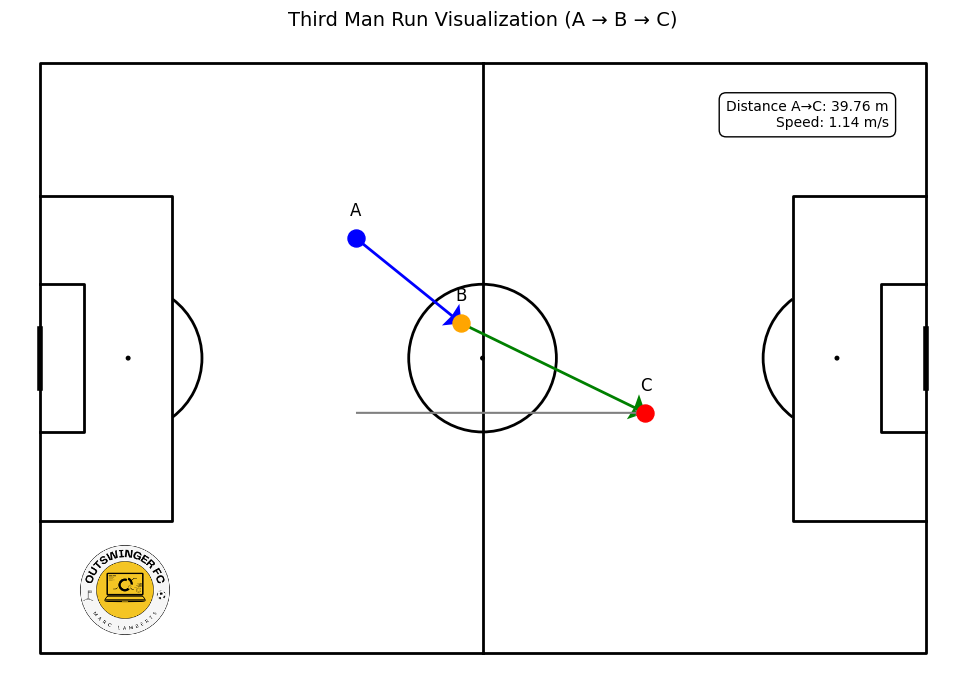
We start by calculating the Euclidean distance between A’s pass location and C’s reception point, which comes out to about 39.75 meters. Dividing that by the time difference gives us a run speed of 1.14 meters per second. We also look at how much progress the ball made toward the goal, called the vertical gain, which in this case is around 0.33 (when normalized to a standard 105-meter pitch). Each of these factors — distance, vertical gain, and speed — is normalized and plugged into a weighted scoring formula. For this example, the resulting value score is 0.468, indicating a moderately valuable third man run.
This process helps quantify the kind of off-ball intelligence that often goes unnoticed. Instead of just knowing who passed to whom, we begin to understand how space is created and exploited. With just a few lines of code and some well-defined logic, we turn tactical nuance into measurable insight — bridging the gap between data and the game’s deeper layers.
Analysis
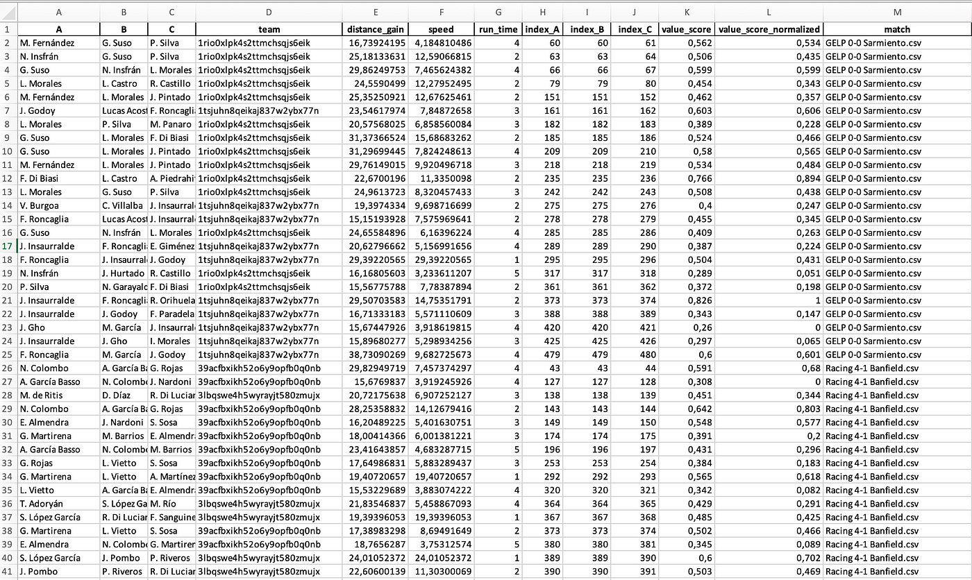
By running the Python code, I get the results of the third-man runs and every player involved. I also calculated a score that gives value to the third man run as to how useful it is. The Excel file that came out of it looks like this:
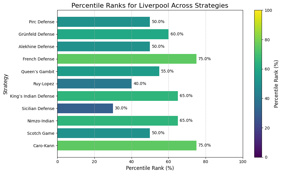
First, let us have a look at the teams with the most third-man runs during these games we have collected:
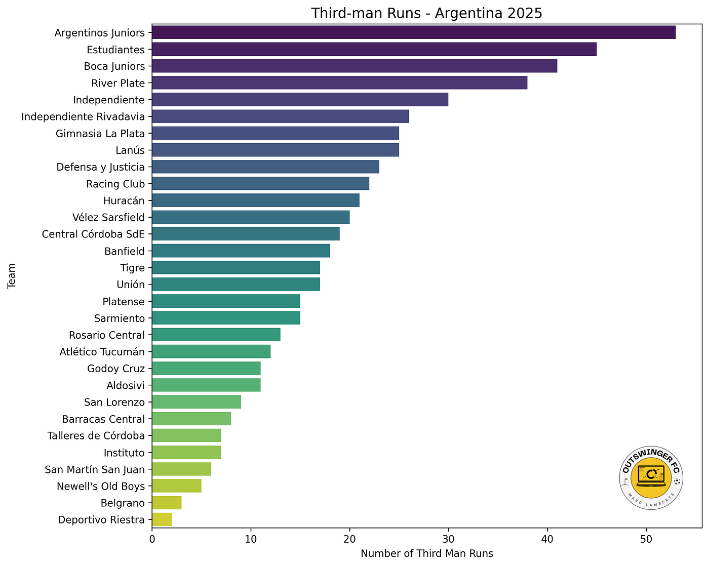
As we can conclude from the bar graph above, Argentinos Juniors, Estudiantes and Boca Juniors have the most third-man runs. Having said that, Newell’s Old Boys, Belgrano and Deportivo Riestra have the fewest third man runs.
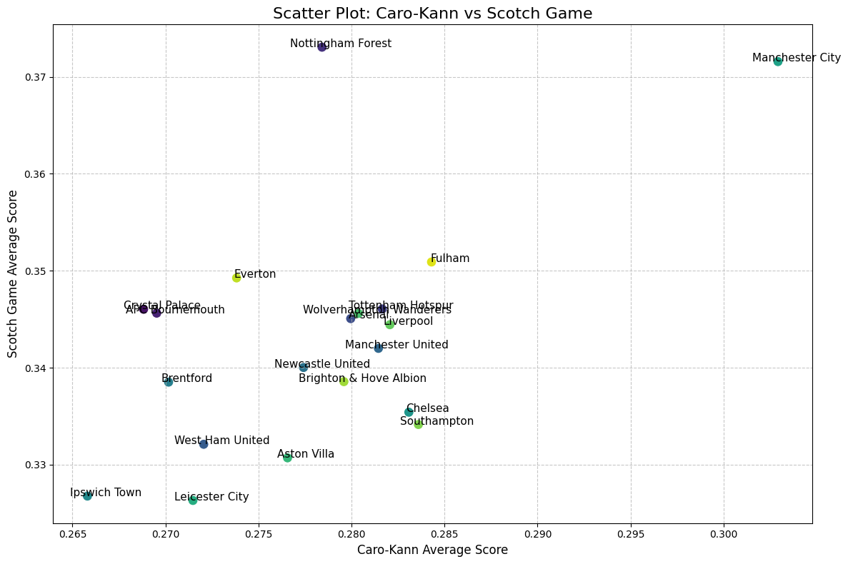
Of course, these are just volume numbers. Let’s compare them to the average value:
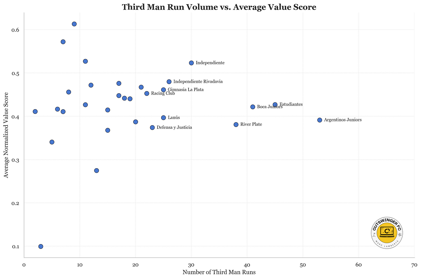
What we see is quite interesting. The majority of the teams have an average value between 0,3 and 0,5 per third-man runs. The more they participate in third man runs, the more the value is even. As you can see, the teams with the fewest have more positive and negative anomalies.
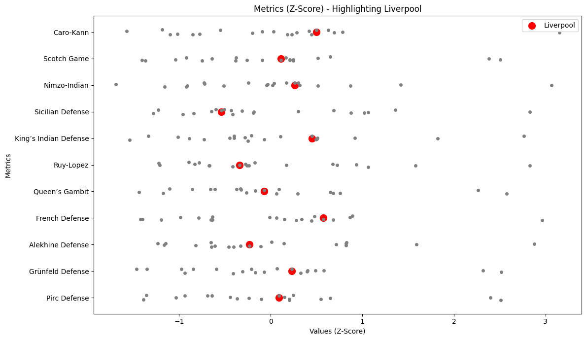
Finally, I want to find the players who are player C, as they are the ones doing the third-man run. I also want to see their value score on average, so we can see how dangerous their runs are.
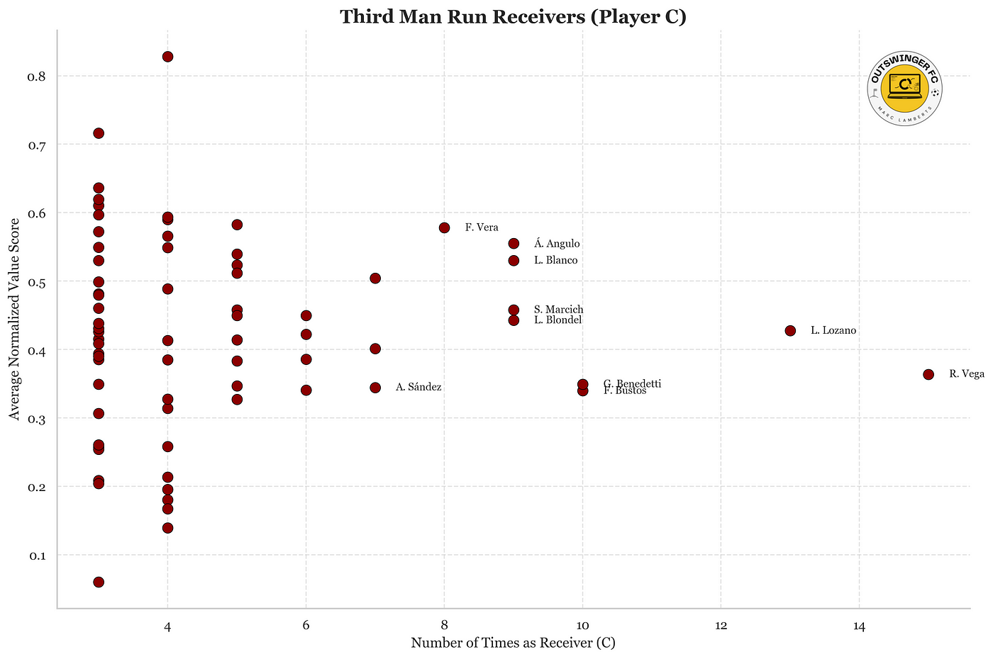
As we can see, there is a similar pattern with how the value is assigned. More third man runs also means a more similar value to their peers. This is very interesting.
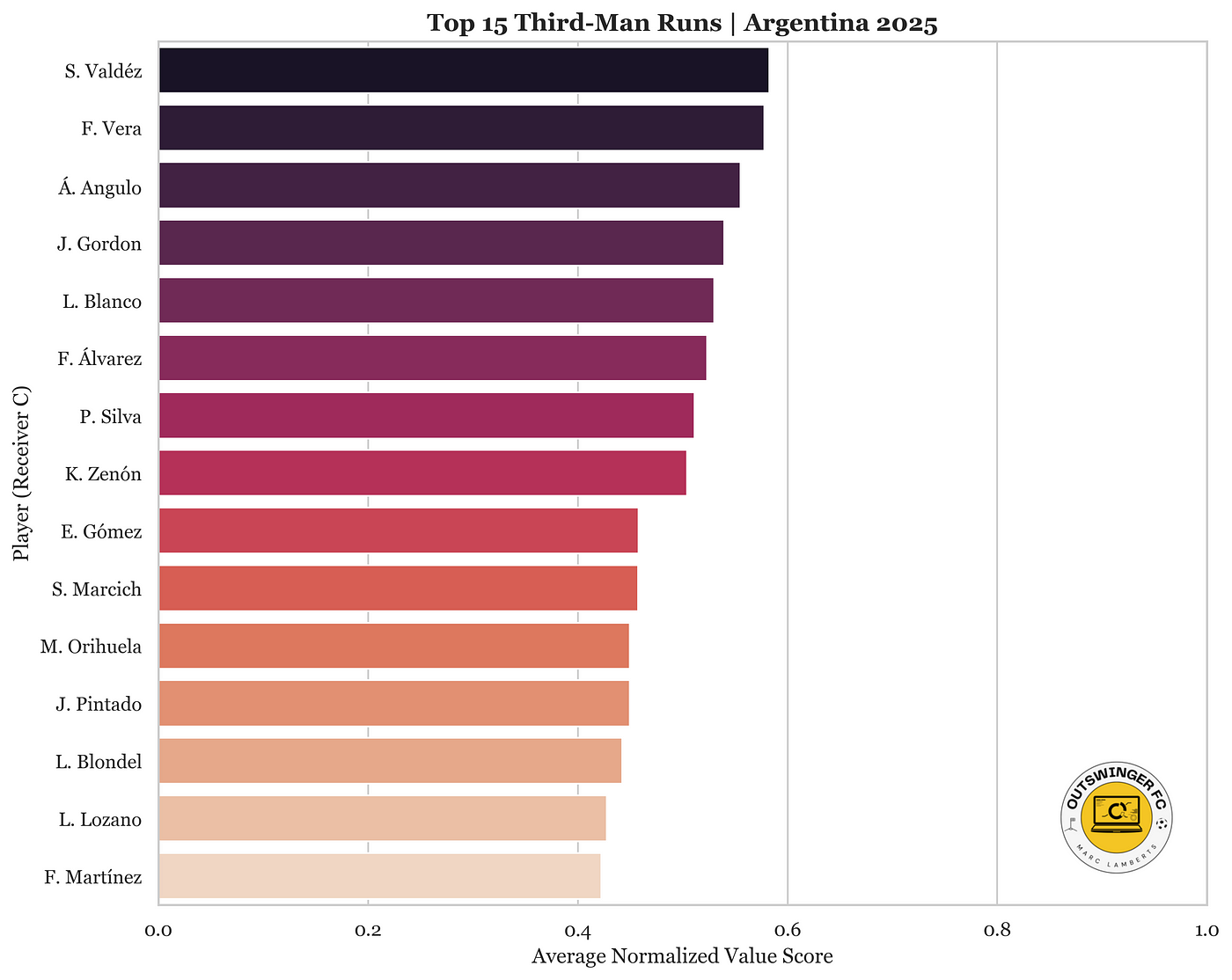
We can see the best players in terms of the value they give with their runs. I have selected only players with at least 5 runs to make it more representative. It’s also important to stress that the league hasn’t been concluded and the data will be different when the season is over.
Now this is a way how we create the metric and analyse it, but how valid is this data actually?
Checks and evaluation
Now I’m going to check whether this is all worth the calculation or that I need to make drastic changes
First, I will look at the feature. The composite score is based on the following: distance (50%), Vertical gain toward the goal (30%) and speed (20%). This seems like a reasonable way to use weights, but I could increase the vertical gain for the values.
Second, looking at the output, I need to ask myself the following questions:
- Are top-scoring actions meaningful? (e.g. fast break runs, line-breaking passes)
- Are short, back-passes scoring low?
- Are there any nonsensical values like 0 distance or negative speed?
Following that, looking at the distribution validation:
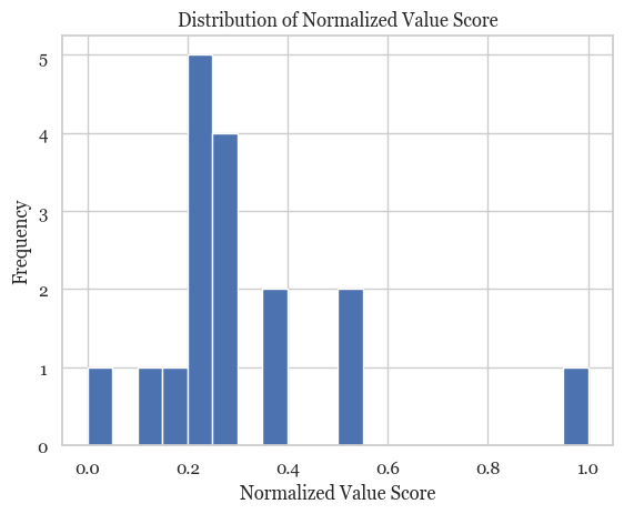
The distribution of normalized value scores for third-man runs appears healthy overall, showing a positive skew with most scores clustered between 0.2 and 0.5. This shape aligns with expectations in football, where high-value tactical patterns — like truly effective third-man runs — should be relatively rare. The presence of a single peak at 1.0 suggests a standout moment, potentially representing a high-speed, long-distance run that created significant forward momentum. Importantly, the model avoids overinflating value, as there’s no unnatural cluster near the top end of the scale, which supports its reliability in distinguishing impactful actions from routine ones.
However, the tight cluster around the 0.2–0.3 range may point to a limited scoring spread, potentially reducing how well the metric separates moderately good actions from low-value ones. This could be a result of either low variability in the input features (like speed or vertical gain) or an overemphasis on distance within the weighted formula. If the score distribution stays compressed, it may make ranking or comparative use of the metric less insightful. Adjusting the weighting or introducing non-linear scaling to amplify score separation could help refine the index for better tactical and scouting utility.
If you liked reading this, you can always follow me on X and BlueSky.