Slowly but surely, this medium account is turning into a more meta-analysis place where I discuss methodology, coding and analysis concerning data specifically used in football. And, honestly, I love that. I always try to be innovative, but that’s not always the right thing to do. Sometimes you need to look back at your process and see if there’s something you can optimise or improve.
That’s something I’m going to do today. I’m going to look at plain outliers in the data for specific metrics and what the case of outlier analysis tells us about the quality of the data analysis. Of course, there are a few problems that arise and I think it’s really good to take a moment and express worries about that.
In this article I will focus on a few things:
- What are outliers in data?
- Homogenous and heterogenous outliers
- Data
- Methodology
- Exploratory data visualisation
- Clustering
- Challenges
- Final thoughts
What are outliers in data?
I was triggered to look deeper into this when I read this blogpost by Andrew Rowlingson (Numberstorm on X)
I want to look at how different calculations influence our way of data scouting using outliers in data, but to do that it’s important to look at what outliers are.
Outliers are data points that significantly deviate from most of the dataset, such that they are considerably distant from the central cluster of values. They can be caused by data variability, errors during experimentation or simply uncommon phenomena which occur naturally within a set of data. Statistical measures based on interquartile range (IQR) or deviations from the mean i.e. standard deviation are used to identify outliers.
In a dataset, an outlier is defined as one lying outside either 1.5 times IQR away from either the first quartile or third quartile, or three standard deviations away from the mean. These extreme figures may distort analysis and produce false statistical conclusions thereby affecting the accuracy of machine learning models.
Outliers require careful treatment since they can indicate important anomalies worth further investigation or simply result from collecting incorrect data. Depending on context, these can be eliminated, altered or algorithmically handled using certain techniques to minimize their effects. In sum, outliers form part of the crucial components used in data analysis requiring an accurate identification and proper handling to make sure results obtained are strong and dependable.
Homogeneous and heterogeneous outliers
Homogeneous outliers are data points that deviate from the overall dataset but still resemble each other. They form a group with similar characteristics, indicating that they might represent a consistent pattern or trend that is distinct from the main data cluster. For example, in a dataset of human heights, a cluster of very tall basketball players would be homogeneous outliers. These outliers might suggest a subgroup within the data that follows a different distribution but is internally consistent.
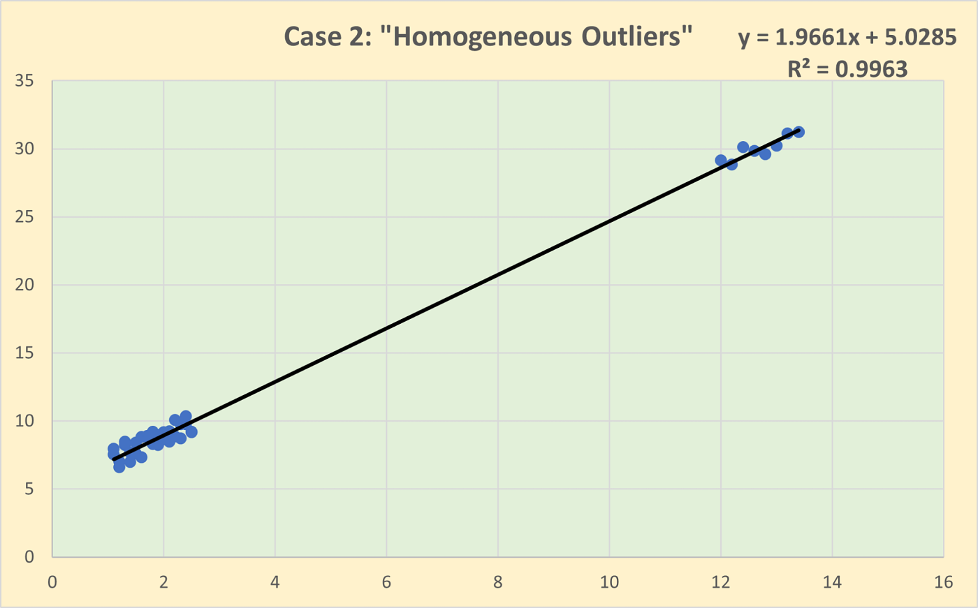
Heterogeneous outliers, on the other hand, are individual data points that stand out on their own, without any apparent pattern or similarity to other outliers. Each heterogeneous outlier is unique in its deviation from the dataset. Using the same height example, a single very tall individual in a general population dataset would be a heterogeneous outlier. These outliers might be due to data entry errors, measurement anomalies, or rare events.
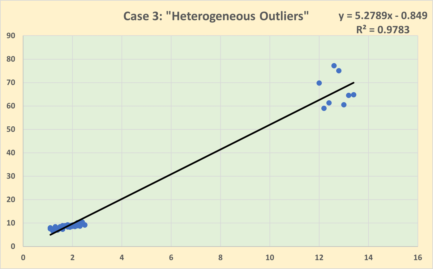
What I want to do in this article is to look at the outliers as described above and see whether using different calculations of deviations has an impact on how we analyse the outliers for the data-scouting process.
Data
The data I’m using for this part of data scouting comes from Wyscout/Hudl. It was collected after the 2023/2024 season and was downloaded on August 3rd, 2024. The data is downloaded with all stats, so we can have the most complete database.
I will filter for position as I’m only interested in wingers. Next to that, I will look at strikers who have played at least 500 minutes through the season, as that gives us a big enough sample over that particular season.

Methodology
To do make sure I can make the comparison and analyse the data in a scatterplot, we need two metrics to put against the x-axis and y-axis. As we want to know the outliers per age group, we will put age on the x-axis and we already have the metric for age.
For the y-axis, we need a performance score and for that we need to calculate the score using z-scores. I have written about using z-scores here:
To calculate the z-scores I will use these attacking metrics available in the database:#Goalscoring Striker
metrics = [“xG per 90”, “Goal conversion, %”, “Received passes per 90”,
“Key passes per 90”, “xA per 90”, “Head goals per 90”,
“Aerial duels won, %”, “Touches in box per 90”, “Non-penalty goals per 90”]
# Adjust the weights for the new metrics as desired
weights = [5, 5, 3,
1, 1, 0.5,
0.5, 3, 1]
So as you can see I’m using Python code to calculate the z-scores and I’m using weighted z-scores to get a specific profile: a goalscoring striker role. In doing so I find the players most suitable for the role and see whether a player is close to the mean or has most deviations from it.
The core of this article is to explore whether the calculation of the deviation has an impact or influence on the outliers. Standard deviation and Mean Absolute Deviation.
Standard Deviation (SD)
Standard deviation is calculated by taking the square root of a value derived from comparing data points to a collective mean of a dataset. The formula is:
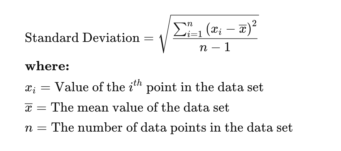
In terms of football, we are going to calculate the mean from the whole dataset with the mean being the most common value of the data metric of PsxG +/-. And with differences from the mean, we are calculating the deviations.
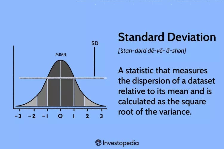
So by doing that, we can see in a more concise manner how a player comes close to the mean or deviates from it. So by using z-scores with standard deviation, it provides a more precise measure of relative position within a distribution compared to percentile ranks. A z-score of 1.5, for instance, indicates that a data point is 1.5 standard deviations above the mean, allowing for a more granular understanding of its position.
Mean Absolute Deviation
The mean absolute deviation (MAD) is a measure of variability that indicates the average distance between observations and their mean. MAD uses the original units of the data, which simplifies interpretation. Larger values signify that the data points spread out further from the average. Conversely, lower values correspond to data points bunching closer to it. The mean absolute deviation is also known as the mean deviation and average absolute deviation.

This definition of the mean absolute deviation sounds similar to the standard deviation (SD). While both measure variability, they have different calculations.
Data visualisations — Standard Deviation
Using a standard deviation we look at the best-scoring classic wingers in the Championship using the standard deviation and comparing them to the age. The outliers are calculated as being +2 from the mean and are marked in red.
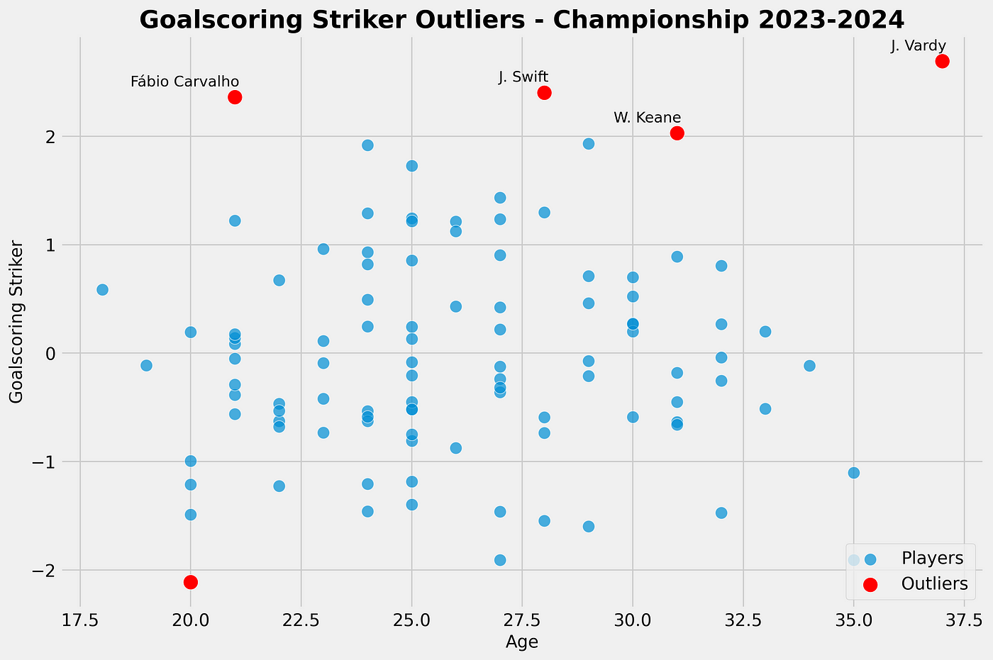
As we can see in our scatterplot, we see Carvalho, Swift, Keane and Vardy as outliers in our calculation for the goalscoring striker role score. They all score above +2 above the mean — and this is done with the calculation for Standard Deviation.
Data visualisations — Mean Absolute Deviation
Using Mean Absolute Deviation we look at the best-scoring goalscoring strikers in the Championship and compare them to their age. The outliers are calculated as being +2 from the mean and are marked in red.

As we can see in our scatterplot, we see Carvalho, Osmajic, Riis, Swift, Tufan, Keane and Vardy as outliers in our calculation for the goalscoring striker role score. They all score above +2 above the mean — and this is done with the calculation for Mean Absolute Deviation. Using this calculation we get more players (3 more) that are further away from the mean.
Clustering — Standard deviation
We can also use our goalscoring striker role and apply clustering to it instead of looking for pure outliers. It has similarities but it is a different method of looking for high-scoring players.

In the graph above you can see the different interesting clusters and see the deviations. For us it is interesting to look at the cluster 3, because these are the ones that positively deviate from the mean.
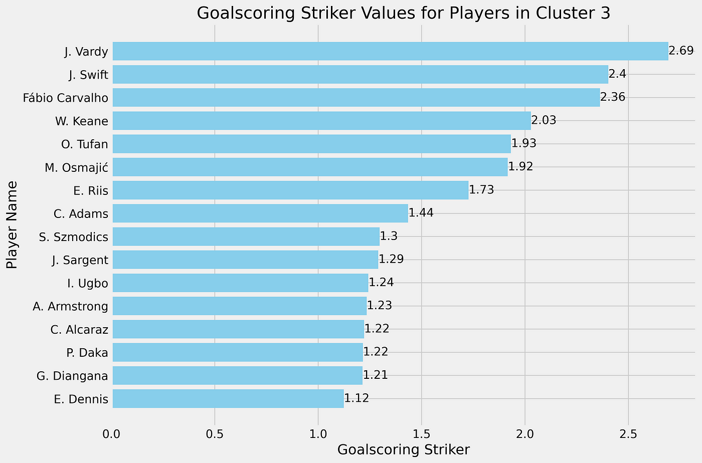
For the clustering in cluster 3, we can see that 15 players are clustered together and might interested to look at. These are obviously clustered to the score calculated with Standard Deviation. The role score varies from +1,12 to 2,69 deviations from the mean.
Clustering — Mean Absolute Deviation
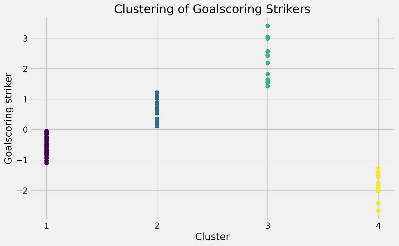
In the graph above you can see the different interesting clusters and see the deviations. For us, it is interesting to look at cluster 3, because these are the ones that positively deviate from the mean.

For the clustering in cluster 3, we can see that 15 players are clustered together and might interested to look at. These are clustered to the score calculated with Mean Absolute Deviation. The role score varies from +1,42 to 3,14 deviations from the mean.
We get a longer list than from the outliers, but via clustering, we can still find interesting players to track according to our goalscoring striker score.
Challenges
One of the challenges of this is that you use different ways of calculating the deviations, but have the same approach to it in terms of outliers. The heterogeneous outliers don’t apply to this as we approach the data in the same way: homogeneous.
I think it’s very interesting that different calculations can lead to fewer or more outliers, but that only has an effect if you focus on the outliers only. You need to be aware of it.
Clustering, however, is a little bit different. We cluster the players that most deviate from the mean together. It gives us a longer list than focusing subjectively on calculating outliers via a significant barrier.
Final thoughts
Most of all this is an interesting thought process. We can use different ways of finding outliers. We can use different calculations of means, using weights on our calculations, use clustering and much more — but these things are always the product of the choices we make when working with data. We must be aware of our own prejudices and biases as to which way we choose to work with data, but different ways can lead to a good scouting process when using data.

Geef een reactie