In media and online scouting reports, we often look at quality. How good is a player at this and that? We look at the quality of the clubs and the leagues. However, we often overlook other important aspects of data scouting, such as consistency and availability.
We often talk about rating strikers and their prime metrics, one of them being expected goals (xG). We look at totals or per 90 metrics, but how can value per 90 if the numbers don’t look at outliers? If you have three high-scoring games, it will cancel out three non-existent games, and still give an average number. So that’s why I today want to have a look at the consistency of strikers by using xG numbers throughout the season.
Contents
- Why do we need this metric?
- Data collection and justification
- Coefficient of Variation
- Methodology
- Low Coefficient of Variation
- High Coefficient of Variation
- Final thoughts
Why do we need this metric?
I’m not exactly creating a new metric, but using a mathematical concept applied to football data. However, there is a use for this in football. Like I said above, we value quality so much, but consistency is key. If you are a consistent scoring player or generating xG consistently — that will mean that players will be valued more for their team.
Using this metric, we can see which players are very consistent in their performances and which players are very inconsistent. We will do this by examining their xG variation throughout the period we are examining.
Corner Possession Index: measuring a team’s possession quality after an attacking corner.
In the past year, I have been looking more and more at data related to set pieces, and corners to be more specific. It…
Data collection and justification
The data used comes from Opta and was collected on November, 22nd 2024. It has event data from the 2024–2025 Eredivisie season up to matchday 12 and is still all raw data. The data that is collected is individual data for each match and not totals, because we need match-level data to measure consistency.
With the data, we can create new metrics and put the data through our xG-model. In doing so, we can calculate the xG per shot, xG per game and xG totals for each individual player and team. I filter for players who have played more than 5 games so we can track the consistency over a longer period.
Coefficient of Variation
The Coefficient of Variation (CV) is a statistical measure that expresses the standard deviation of a dataset as a proportion of its mean. It is often used to assess the relative variability or consistency of data, particularly when comparing datasets with different units or means.

For instance, when analysing performance metrics, CV provides insight into how consistently values are distributed around the average. It is particularly useful for comparing datasets where absolute values may differ significantly but relative variability is of interest. The CV is expressed as a ratio or a percentage, making it a versatile tool in understanding proportional variability.

From this formula, we get a result. This result gives a high or low CV. This can have two meanings:
- Low CV:
- Indicates that the data points are tightly clustered around the mean.
- Suggests greater consistency or predictability.
- Example: A CV of 0.1 (or 10%) in a soccer player’s performance metric (e.g., goals per game) indicates stable performance over time.
- High CV:
- Indicates that the data points are more spread out relative to the mean.
- Suggests greater variability or inconsistency.
Methodology
As said above, we first need to calculate the xG values for the whole Eredivisie in the 2024–2025 season. I’ have a model that converts shot values to shot values with xG values based on 400.000 shots taken. We then get a result.

From having this information which was put through R, we will then focus on the critical part of getting to the CV: calculating the mean and standard deviation. I will use Python to run the calculation and it’s focused on having the PlayerId and the xG value.import pandas as pd
# Step 1: Load Excel file
df = pd.read_excel(‘EREXG.xlsx’)
# Step 2: Extract date from the timestamp
df[‘Date’] = df[‘Date’].str.split(‘T’).str[0] # Extract everything before ‘T’
# Step 3: Calculate CV for xG grouped by Player and count the number of games
cv_results = df.groupby(‘PlayerId’).agg(
Mean=(‘xG’, ‘mean’),
StdDev=(‘xG’, ‘std’),
Games_Played=(‘Date’, ‘nunique’) # Count unique dates
).reset_index()
# Calculate Coefficient of Variation (CV)
cv_results[‘CV’] = cv_results[‘StdDev’] / cv_results[‘Mean’]
# Step 4: Rank players by CV
cv_results = cv_results.sort_values(by=’CV’) # Ascending: smaller CV = more consistent
# Step 5: Save results to an Excel file
output_file = ‘Player_CV_Results_With_Games.xlsx’ # Specify the output file name
cv_results.to_excel(output_file, index=False)
print(f”\nResults saved to {output_file}”)
As a result, I get an Excel file that shows me the PlayerId, the mean, the standard deviation and the CV. The matches played are also included. Now we have the framework on which we can start analysing.
Low Coefficient of Variation

In the bargraph above you can see the top 15 players with the lowest coefficient of variation. This means that they have the least variability of their xG performance and therefore are consistent in their games through the first 12 games of the season.
High Coefficient of Variation

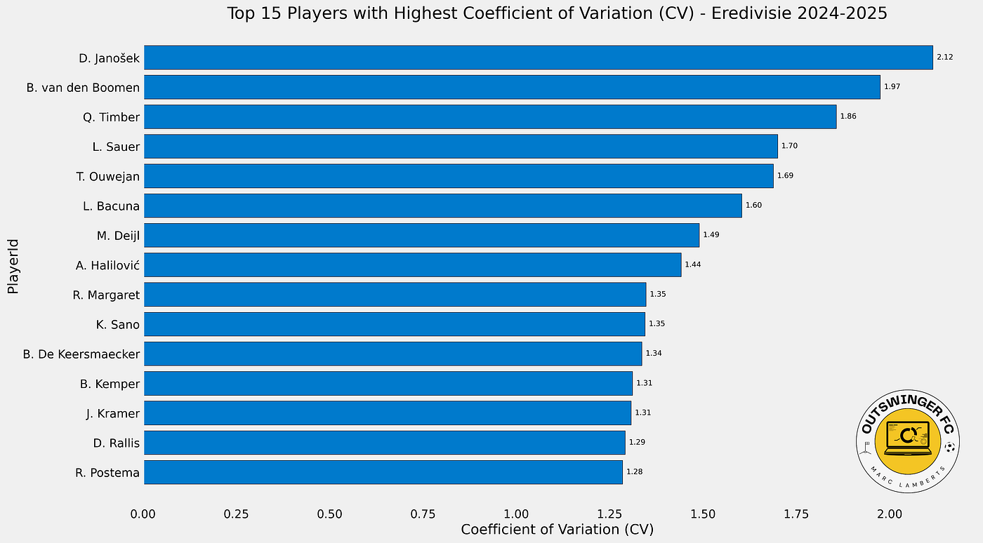
In the bargraph above you can see the top 15 players with the highest coefficient of variation. This means that they have the most variability of their xG performance and therefore aren’t consistent in their games through the first 12 games of the season.
This can have several reasons why these players are featured in the low CV or in the high CV. The most common are position, how the team performs, how strong the opposition is. However it shows consistency or inconsistency, which is the aim of this metric.
Final thoughts
It has been an interesting thought experiment to look at consistency across a series of games for players in the Eredivisie, but there are a few things that I would different the next time:
- Look at minutes played rather than matches played as it gives a better idea of on field actions
- Filter for positions, this will be more useful for attackers than for defenders
- Get a database that looks at a longer period to make a representative judgement of consistency.

The next time I would also like to answer the question whether consistency is also a matter of playing many games. In other words does it even out over time and you become more consistent? From my small sample size it looks like it as you can see in the scatterplot above.

Geef een reactie