

Expected goals. You might think oh no here we go again, but I think it might be the one metric that has become part of normal conversations, without actually knowing the power or versatility of it. That also means we often talk about expected goals or xG and make wrong assumptions/conclusions. This can lead to a completely distorted point of view and discredit the work data people do in sports.
So, where am I going with this? In my opinion, xG can be used in multiple ways — if the context is right. I was looking for a way to see whether I could see that the quality of the chances or likelihood of a shot being converted into a goal would be different according to game state. In this article, I will break down how I use event data to calculate xG and how to use game state adjusted xG scores.
What is expected goals?
There are various explanations, but I thought the one The Analyst gave is pretty accurate:
“Expected goals (or xG) measures the quality of a chance by calculating the likelihood that it will be scored by using information on similar shots in the past. We use nearly one million shots from Opta’s historical database to measure xG on a scale between zero and one, where zero represents a chance that is impossible to score, and one represents a chance that a player would be expected to score every single time.
We know that a chance from the halfway line isn’t as likely to result in a goal as a chance from inside the penalty area. With xG, we can give numbers to these scenarios. For example, suppose the chance from inside the box is assigned an xG of 0.1. This means that a player would, on average, be expected to score one goal from every ten shots in this situation or 10% of the time.
The terminology may be new, but these phrases have been used by football fans and commentators for years before xG was introduced — “he scores that nine times out of ten” or “he should’ve had a hat-trick today”.”
Data collection
As I have expressed before, we will work with event data and that is in my opinion one of the best ways to work with metric creation or metric development.
For this, I am using Opta event data and specifically the shot data. The event data means that I will use the x and y coordinates of specific action to calculate shots-related metrics that will help us in this analysis.
I have collected the data from Opta and looked at a full season of the Allsvenskan, the top tier in Sweden, in 2023. By having a complete season, we can have a more accurate analysis and conclusion regarding the data. The data was collected on February 25th, 2024.
Methodology
Calculating expected goals (xG) in football entails a meticulous process that transforms raw event data into probabilistic assessments of scoring opportunities. At its essence, xG analysis aims to quantify the probability of a particular event, like a shot or a pass, culminating in a goal. This undertaking commences with the comprehensive collection of detailed data on various match occurrences, encompassing shots, crosses, and defensive actions. Each event is subjected to meticulous scrutiny, with variables such as its location on the pitch, the nature of the event, and the presence of defensive pressure meticulously considered.
Following the data collection phase, the next step involves feature engineering, where raw metrics are refined into meaningful predictors of goal probability. For example, factors like the distance from the event location to the goal, the angle of the shot, and the number of defenders between the shooter and the goal are all pivotal in influencing the likelihood of scoring. These features serve as the basis for training statistical or machine learning models, which leverage historical data to predict the probability of a goal for each event.
In real-time during matches, the trained models are then applied to fresh event data, generating expected goal values that range from 0 to 1 for each scoring opportunity. Elevated xG values indicate a higher probability of scoring from a specific event, while lower values suggest less promising prospects.
Expected goals
After we put the collected data into our expected goals model, we will get the xG values with the players and the locations of the shots. It will look something like this:
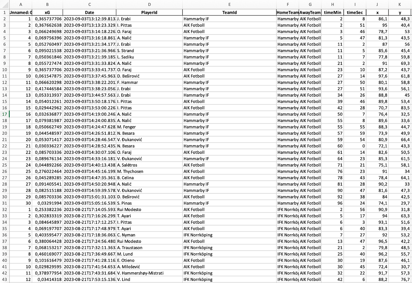
We have different columns in our Excel file after it comes out of the model. The most important is to see which player of which team has what specific xG score of the shot they have taken.
With the expected goals per shot, we can of course calculate the xG for that whole game, series of games, or the whole season. We can also calculate the average xG per shot, but what happens a lot too, is that we can make shot maps out of it, xG plots, and bar graphs — this information can help you a lot going forward in your data analysis.
Categories
In this document or in most xG-generated data, we can make a distinction between different categories with data:
- Open play: All shots that come as a result of open play. This can be from a build-up or from a counter-attack.
- Set pieces: all shots as a result of dead ball moment. Corners, direct free kicks, indirect free kicks, and throw-ins.
- Non-penalty: xG that comes as a result of everything that isn’t a penalty. Penalty xG is very high and always the same, which means it can screw with the representation of the data.
- Time: in which parts of the game is xG generated. In other words: what can we tell about xG by looking at the periods throughout the games?
- Bodypart: is the shot done by the left foot, right foot, head or other body part?
Game state xG
The categories mentioned above are all valid in doing research into what xG can do, but there is another category that can help us in a way the others do not: game state.
With game state, I mean what the score is and whether a player/team is leading, trailing, or drawing. My central question is: is xG influenced by the game state of that specific match?
To accurately research that, I’m going to take a specific player and look at the following aspects:
- Expected goals — Total
- Expected goals while leading
- Expected goals while drawing
- Expected goals while trailing
By looking at that, I can conclude shot locations and probability based on game state.
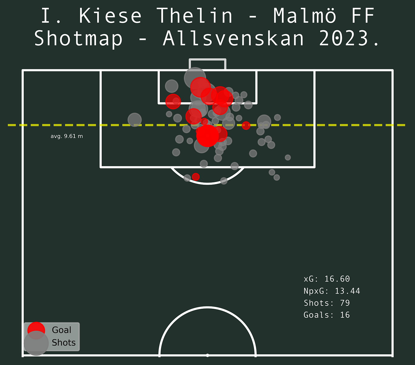
In the shot map above you can see the total number of shots of 79 in the whole season with a corresponding xG of 16,60. The average distance to goal is 9,61 meters.
If we want to see how this varies or is influenced by the game state, we first look at the game state when Malmö are leading.
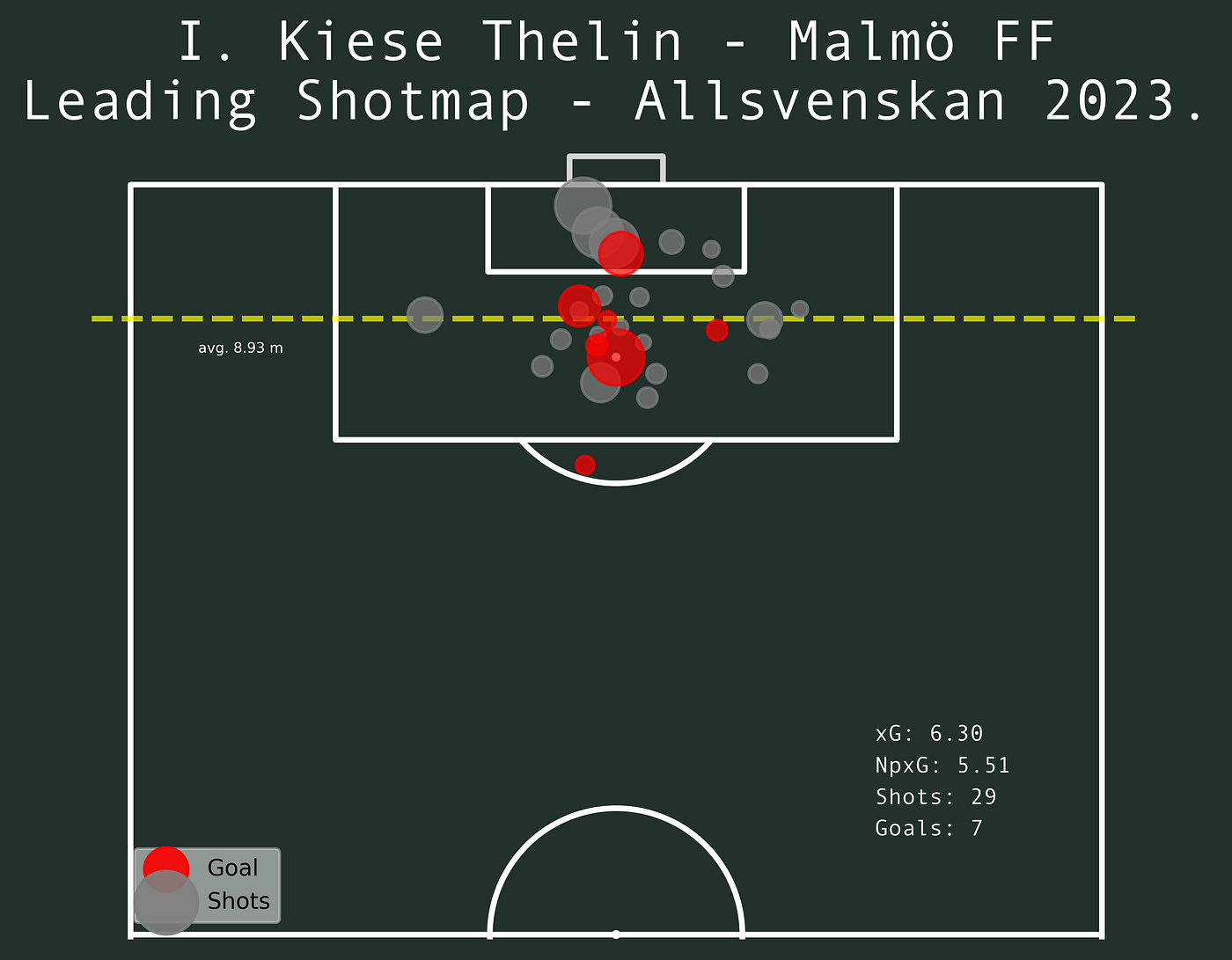
When Malmö are leading, Kiese Thelin has had 29 shots with an xG of 6,3. The average distance is 8,93 which is closer to the goal than the total average of shots during the 2023 Allsvenskan.
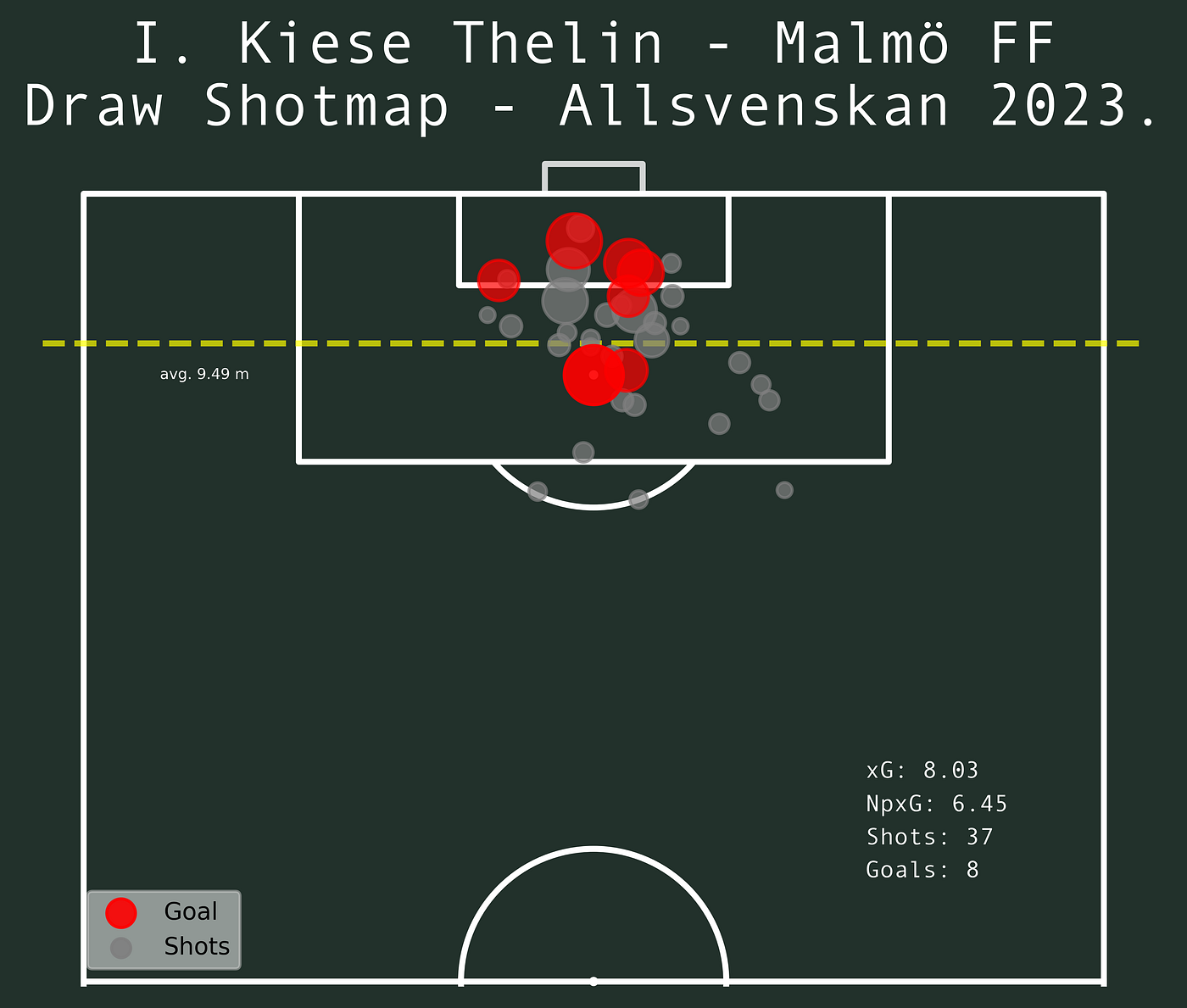
When Malmö are drawing, Kiese Thelin has had 37 shots with an xG of 8,03. The average distance is 9,49 which is closer to goal than the total average of shots during the 2023 Allsvenskan, but only slighter. So there are more shots taken and from a great distance.

When Malmö are trailing, Kiese Thelin has had 13 shots with an xG of 2,27. The average distance is 11,51 which is further away from the goal than the total average of shots during the 2023 Allsvenskan. Fewer shots hav been taken, but the distance is bigger, which can lead to the conclusion that he shoots earlier and farther away from the goal.
In general, we can say that this player specifically shoots more and scores more when the teams are drawing. Then the leading game state comes, but with the sidenote that the shots are closer to goal and therefore generate more xG per shot.
Challenges
There are of course challenges and things to improve going forward. The first thing is to look at your expected goals model. Mine has been trained with 400.000 shots in the simulation, but it’s very focused on the shooter and not on the other factors. This also means that the models by Wyscout, Opta, and Statsbomb are more complete, and consider more things. You need to be aware of the quality of the data you are working with, but also on the level of methodology you are applying to your research.
Another challenge is to adjust the scores and quality of the players and teams. Kiese Thelin played for Malmö in the 2023 season and they were the champions dominating many of the games. This also means that the time that they were trailing was considerably less than for example a player playing for a team at the bottom.